A clinician with a critically ill newborn needs an answer within the shift, not within the week. Rapid whole-genome sequencing exists for exactly this case, and the constraint on it is that it runs at a handful of centers on an instrument costing several hundred thousand dollars at minimum. Most infants would never get it. An answer produced on something small enough to sit in a hospital rather than a reference lab is a different clinical object than the same answer produced somewhere else a week later.

On a more speculative note, we think the throughput our architecture allows may be what brings us a step closer to generating the data necessary for a general genotype-to-phenotype model. Every genomics dataset we have is small by the standards of the models that would want to consume it, and the reason is cost per sample, not interest. If sequencing gets cheap (and fast) enough, population-scale data stops being a funding decision and becomes the default. Imagine sequencing ten thousand fruit flies and mapping every one of those genomes to their physical expression. It would allow for a direct representation of their physical expression to be generated purely off their genome and a sufficient epigenomic world model. Taking this a step further, imagine creating synthetic organisms to farm organs for transplants or engineering microorganisms for medicine and industry. We think this would change the world.

In a conventional platform the wash does two jobs. It clears the previous cycle’s chemical components so the next base can be read, and it acts as a synchronizer, holding every copy in a cluster on the same clock. Because of that second job, cycle time is bounded below by the fluidics, and everything downstream inherits that bound.

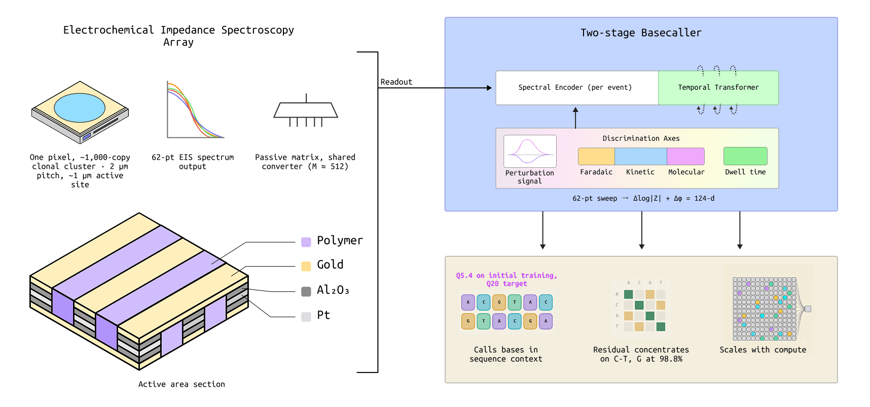
Read the base without a label and both jobs disappear at once. There’s nothing to clear, so all four nucleotides sit in the reaction simultaneously and the polymerase runs continuously instead of one base per cycle. What ECSEQ-0 reads is the electrical disturbance the incorporation itself makes. As a polymerase extends a surface-bound strand, the impedance of the electrode-electrolyte interface shifts, and that shift depends on which base went in. Measuring it by impedance spectroscopy at each pixel is the whole measurement. Nothing is labeled, nothing is imaged, nothing is exchanged.

Every pixel stacks a top gold electrode over an anodized Al₂O₃ dielectric over platinum. Gold anchors the DNA and carries the molecular signal, and platinum is the impedance transducer. Two metals rather than one is what makes frequency decomposition available at all. The two interfaces relax on different timescales, so their contributions separate across frequency instead of summing into one indistinguishable response. The array is addressed passively over row and column lines, with no per-pixel circuitry and no basecalling logic on chip.

A single molecule doesn’t move the impedance enough to detect, so each landed fragment is copied in place by isothermal bridge amplification: a surface-bound strand arches over, hybridizes to a neighbouring primer, gets extended, and denatures into two bound copies. Iterate on this and we get a clonal cluster of roughly a thousand identical copies over one pixel. What the sensor reads is the ensemble average of a thousand polymerases doing the same thing at the same time, and amplification runs at the same 65 °C as sequencing, on the same primer lawn the electrode already needs.

Anyone who’s followed electronic sequencing is thinking about homopolymers by now, and they should be. A semiconductor sequencer that reached market at scale infers run length from the magnitude of one summed signal, so telling five identical bases from six means resolving a noisy continuous value into an integer, and independent benchmarking made that its characteristic error mode. That failure comes from being flow-limited: one nucleotide species is dispensed at a time, so a run collapses into a single event.

ECSEQ-0 was never flow-limited. All four nucleotides are present continuously, so each incorporation is a separate kinetic event spaced from its neighbours by the polymerase’s own timing, and a homopolymer should read as a train of dwell-resolved events rather than one smeared magnitude. This is a testable prediction and an open problem for us.

The incorporation perturbs the interface along three physically distinct axes. A kinetic band from 100 Hz to 10 kHz, where the platinum double layer dominates, carries the base-dependent time the polymerase spends in its closed conformation. A molecular band in the 10 to 100 kHz tail carries the dielectric and dipole coupling of the incorporated nucleotide to the gold. And a faradaic band at 20 to 90 Hz carries base-dependent charge transfer near the guanine oxidation onset, which is what breaks the A/G pair the other two leave tangled.

It’s worth seeing why no single axis carries the call. Dwell time is the most intuitive of the three and the easiest to overrate. The four distributions overlap heavily, and there’s no threshold you can draw that separates them.

The spectrum has the same problem in a different form. Charge-transfer resistance varies roughly 25% pixel to pixel from fabrication and functionalization tolerances alone, which swamps anything base identity contributes. So the model never sees a raw spectrum. It sees the change between the incorporation and that same pixel’s quiescent baseline, in polar form this is a log-magnitude change and a phase change at each frequency.

Removing the wash isn’t free, and the bill comes due in read length. Two independent mechanisms bound it, and the effective limit is the tighter of the two.

The first is geometric and easy to picture. An electrode’s field doesn’t reach far into an electrolyte, because dissolved ions rearrange to cancel it within a few nanometres. Each base carries the polymerase active site 0.34 nm further out, so after roughly nine bases at the ionic strength an active polymerase requires, the event falls outside the region the electrode can sense. The most dilute compatible buffer stretches that to almost thirty.

The second is coherence, and it’s the tighter one. The wash was the synchronizer. Without it, each of the thousand copies performs its own random walk in position, and the ensemble smears.

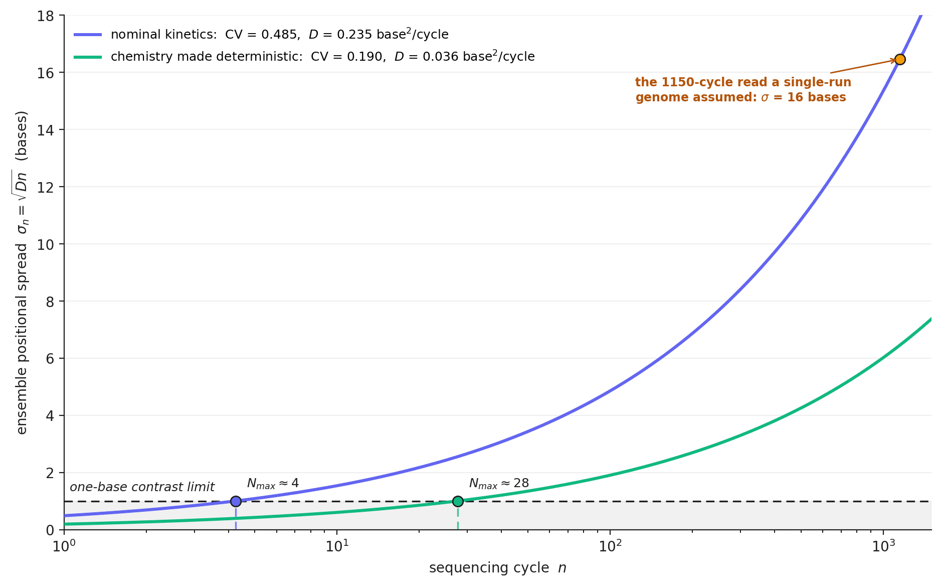
So this is a short-read architecture, and it’s short for two reasons rather than one. Lifting either bound alone buys nothing. The target is smaller than it sounds, though, because a read needs to be mappable, not long: from about nine bases to the 20 to 25 base floor that unique placement against a 3.2 Gb reference requires. A factor of three, not the three orders of magnitude that would put us in competition with nanopore on read length. That’s a tractable engineering bet, and it’s also where most of our risk sits. If single-pixel validation can’t clear the mapping floor at a polymerase-compatible ionic strength, the whole-genome application closes and this stays a targeted-panel device.

Now let’s get down to the numbers.

Read length doesn’t appear in the base rate at all. It enters only through the run count, through how many times the fixed overhead of sample preparation has to be paid. So closing a genome in a single run is just a parallelism condition: pixels, times read length, times occupancy yield, exceeds the bases you need.

Two things fall out of that. The architecture-independent figure of merit is an areal base rate of about 2.1 × 10⁶ bases per second per mm², quoted at 2 µm pitch and full occupancy, depending only on pixel count and polymerase turnover and surviving every correction to read length. And once a configuration closes a genome in one run, sequencing occupies well under 1% of wall-clock time: at a 30-base read, about 3.5 seconds of sequencing against a 35-minute library prep.

That result is deliberately anticlimactic.

Time-to-result becomes time-to-prep. It’s an array-area claim and a sample-prep claim, not a sequencing-speed claim, and neither is where our technical differentiation lies. Prep is a borrowed primitive, and the most concrete lever on it is switching from conventional fragmentation and ligation to tagmentation, where rapid kits report hands-on times around ten minutes.

The area is the harder half. At a 30-base read and a 0.5 µm pitch, closing a 30× genome in one run needs roughly 2,200 mm² of active area. That’s within the reticle-stitched area of a single 300 mm wafer, about 2.4× the 900 mm² panel scale our throughput analysis uses as its reference point, and several hundred times the 3.69 mm² of the full-spec die we’ve actually designed for experimentation. It also assumes reads clearing both Q20 accuracy and long enough to mapped to the desired genome.

The readout figures here are quoted at panel scale, 900 mm² at 2 µm pitch, rather than at the larger single-run area above. Reading its 2.25 × 10⁸ pixels at cadence needs about 3.4 × 10⁹ spectra per second, which one front-end per pixel would never deliver at a cost consistent with a passive array. Code-division multiplexing does: about 512 pixels per converter and roughly 67,000 converters, which is a big data-acquisition format, but a buildable one. It depends on an analog baseline nuller, standard in SQUID readouts, to cancel the quiescent baseline before digitization. Without one, the buildable depth collapses roughly thirtyfold, to about 250 pixels per converter, which is under the 512 the scheme needs.

Either way, none of this touches the active area, and all of it sits on the cost-and-capability curve that fluidics does not.

Every number here comes from a physics simulator that models the chain from polymerase kinetics through gold and platinum transduction, dephasing, and correlated noise. Those numbers answer the narrower question that has to come first: whether the three-axis signal, as modeled, carries enough information to separate four bases, and whether a decoder can recover it. An instrument whose signal can’t be decoded in principle isn’t worth fabricating.

The answer is yes, we’ve found, with a specific and instructive caveat.

The per-event encoder, calling each incorporation in isolation, reaches 50.1%. The temporal stage lifts that to 71.2% per base, or Phred Q5.4, on 30-base reads. Our goal production floor is Q20, which is 99%. We’re roughly thirty times too error-prone at short read lengths for whole-genome mapping.

So that’s the honest state of our platform. We have a decoder that works on simulated data, with extensive plans for hardware validation and some clever engineering left to close the gap.

The error has structure, and that’s our strongest indicator of success. The residual isn’t spread evenly across four bases the way noise would be. Guanine is called at 98.8% and the A↔G purine pair is essentially resolved, accounting for 1.3% of all errors and under 0.4% of all calls. The limiting channel is the pyrimidine pair instead, which the faradaic axis doesn’t currently target. Thymine is called correctly in only 45.0% of cases, and C↔T is the single largest error channel. Cytosine sits at 65.2%, and adenine at 75.3% loses predominantly to thymine rather than to its fellow purine. That localizes the shortfall to a missing discrimination axis rather than to a noise floor, which we think is a far more tractable thing to have to change.

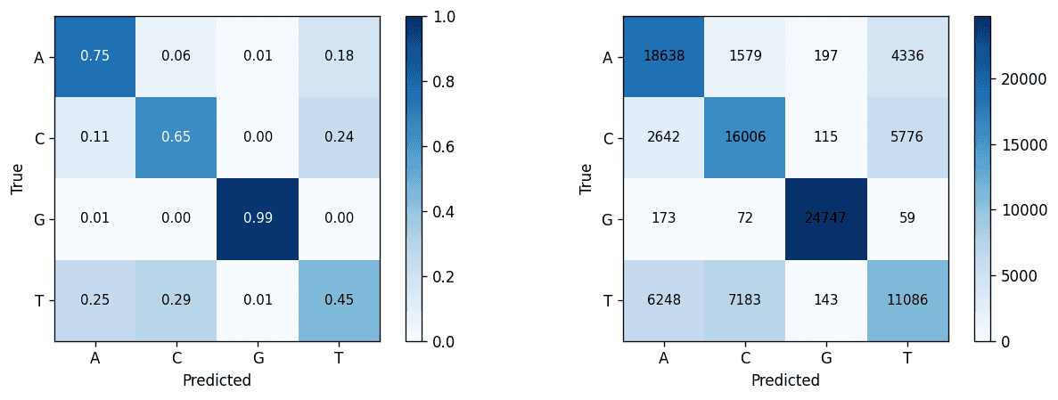
Structured error does carry a cost. Because it’s systematic rather than random, coverage doesn’t average it away, and the same miscall recurs at the same reference position across independent reads. Only added information fixes it, which makes a fourth discrimination axis for the C/T pair the decisive route, and the clearest single piece of physics to complete this puzzle.

Context is our largest demonstrated lever. The same architecture reaches 89.6% per base at 100-base reads, where the per-event encoder also rises to 76.7%. That isn’t a supported operating point, since 100 bases sits outside both read-length bounds. What it measures is decoder capacity given abundant context, which is exactly what an extended sensing envelope would supply. Read length and accuracy are one problem, not two.

There’s direct precedent on the decoder side. Successive nanopore basecaller architectures moved read accuracy into the high eighties and low nineties on a physical signal that never changed, with the conditional-random-field decoder outperforming CTC. That’s the curve we’re claiming to be on, and it’s the concrete manifestation of our core thesis that AI is the instrument to be modulated in our architecture, not the semiconductor process development. Our chip is passive and fixed and reports the state of its own surface, but everything that turns that report into an answer is a model. Nobody can upgrade a shipped flow cell’s chemistry by software.

Both read-length bounds are sequencing problems specifically. They exist because synthesis carries the event away from the electrode, and because a thousand copies of a growing strand can’t stay in step without a clock. Most things worth measuring hold still. A hybridized target, an antibody-antigen pair, a redox-active metabolite: each sits inside the sensing envelope, and none are read-length-limited at all. The same array, the same multi-axis physics, and the same class of decoder read them, with pitch and active-site size chosen to match the analyte. Because the readout is continuous and electrical, they can run as long-duration monitoring rather than single-shot tests.

That’s the reason to build an instrument and not a sequencer. Sequencing is the hardest application we could find, chosen because the signal is weak, the event is fast, and the answer has to be one of four. If the architecture holds there, label-free pathogen detection, targeted molecular panels, and continuous biomarker monitoring are easier chips on the same reader, inheriting the same decoder and the same simulator-and-calibration flywheel. The cost argument has the same shape: to first order the per-genome cost is chip cost divided by reuse count, plus prep, and neither term is a single-use flow cell.

Our immediate work is hardware: fabricate a single pixel, run the calibration pair, recalibrate the simulator against the real interface, and fine-tune the basecaller from its existing checkpoint onto real reads. On the model side the next step is event segmentation, since every accuracy here assumes one delimited spectrum per incorporation and a real device delivers an unsegmented stream.

The array is the part that has to be built once. It’s fixed, passive, and deliberately cheap, and its whole job is to report the state of its own surface. The chip that reads a panel today should read it better next year, and read something else entirely the year after, with nobody returning to the fab in between. None of that is close yet, but it’s far off for reasons we can enumerate, in an order we can attack, and the first one is a single pixel experiment.